Chapter 20
Quantum Computing and Cryptography
20.2 Quantum Algorithms
20.3 Issues in Quantum Computing
20.4 Quantum Cryptography
20.5 Cryptography in the Quantum Era
A.1 Assumptions
A.1.1 Encryption
A.1.2 Knowledge of Attacker
A.1.3 Authentication with Symmetric Key and MACs
A.1.4 Hash Functions
A.1.5 Digital Signatures
A.1.6 Key Management and Random Numbers
A.2 Principles
B.1 Common Data Formats
B.1.1 English Alphabet
B.1.2 Printable Keyboard Characters
B.1.3 Binary Data
B.1.4 ASCII
B.1.5 Hexadecimal
B.1.6 Base64
B.2 Conversions using Linux
B.3 Conversions using Python
C.1 Organisations in Cryptography and Security
C.1.1 National Institute of Standards and Technology
C.1.2 International Association for Cryptologic Research
C.1.3 Australian Signals Directorate
C.1.4 National Security Agency
C.1.5 Government Communications Headquarters
C.1.6 Institute of Electrical and Electronics Engineers
C.1.7 Internet Engineering Task Force
C.2 People in Cryptography and Security
C.2.1 Diffie, Hellman and Merkle
C.2.2 Rivest, Shamir and Adleman
C.2.3 Alan Turing
C.2.4 Claude Shannon
C.2.5 Hedy Lamarr
C.2.6 Phil Zimmermann
C.2.7 Other People
File: crypto/quantum.tex, r1971
This chapter contains brief notes on concepts related to quantum computing and quantum cryptography. The intention is to be able to understand the role of quantum computing with respect to attacking ciphers, as well as the security mechanism quantum cryptography provides.
Disclaimer: These are very rough notes. A lack of time and in-depth understanding of quantum computing on my part means there are likely errors, some parts may be confusing, and the presentation is quite poor (mainly definitions which are not actually definitions; insufficient examples or diagrams). However it should be enough to gain an idea what role quantum technology plays in cryptography. The plan is to update the content after feedback from others.
This information comes from a collection of resources, including Wikipedia pages, news articles and videos. Some, but definitely not all, of those sources are, in no particular order:
- https://quantum.country/
- https://blogs.iu.edu/sciu/2019/07/13/quantum-computing-parallelism/
- https://arxiv.org/abs/quant-ph/0507023
- http://www.columbia.edu/~jpp2139/decoherence-superconducting-qubitsWEBv2.pdf
- https://www.ibm.com/quantum-computing/
- https://qiskit.org/textbook/preface.html
Presentation slides that accompany this chapter can be downloaded in the following formats: slides only (PDF); slides with notes (PDF, ODP, PPTX).
20.1 Quantum Computing
Definition 20.1 (Quantum Technology). Emerging technologies that build upon concepts of quantum physics, especially superposition and entanglement. Includes quantum computing and quantum cryptography.
Note that before quantum physics we had “classical” physics. Similar, we will differentiate between quantum computers and classical computers (those that we know and use everyday). Also, roughly, quantum physics and quantum mechanics means the same thing in this discussion, and we refer to quantum-mechanical systems.
To arrive at an explanation of a quantum computer, as well as quantum cryptography, we will step through some of the basic principles/ideas. First we will look at how information is represented in
Definition 20.2 (bit). Binary digit, 0 or 1, as the basic unit of information in classical computers. For example stored as electric charges in capacities or with magnets in hard disks. Communicated with electrical or optical pulses. A bit has two states: 0 or 1.
A bit is defined, in an informal manner, just for reference.
Definition 20.3 (qubit). Quantum bit has states represented in a quantum-mechanical system. The state of a qubit is a vector. A qubit has two basis states, and , but many possible states in between. Often represented using subatomic particles such as electrons or photons.
The key distinguishing feature of qubits compared to bits is that qubits have many possible states, not just 0 and 1.
The notation used is not so important here; it is just a short way that we can identify the two basis states which are similar to bit 0 and bit 1. We will see next how the qubit is expressed when in the “in between” states.
Definition 20.4 (Quantum Superposition). Any two (or more) quantum states can be added together to form another quantum state. That result is a superposition of the original states.
Superposition is a concept seen in other systems, but quantum superposition is the main concept that delivers powerful innovations with quantum computers.
Example 20.1 (qubit Superposition). Basis state is like bit 0. Basis state is like bit 1. The state is an example of a superposition of the two basis states, and forms another state of the qubit. Another example state is . In general, a superposition state is , where .
You may think of the concept as superposition as follows. A classical bit has the value 0 or 1. A qubit has the value of 0 or 1, or a value that is both 0 and 1 at the same time.
An important point is that the weights, and , can be controlled. This is the key part of how qubits are used in calculations, as next we see that measuring a qubit returns 0 or 1 with some probability.
Definition 20.5 (The Measurement Problem). Measuring a qubit gives the bit 0 with probability and bit 1 with probability . After measurement the qubit enters (collapses into) the basis state.
There are two important issues about measuring a qubit. First, the result will either be 0 or 1. However when the qubit is in a superposition state of , then we don’t know in advance which value will be output from the measurement. But we do know that with probability it will be bit 0 and with probability it will be bit 1. By controlling the weights, and , we can increase the probability that a useful output will be measured.
The other issue is that upon measurement, the qubit reverts to one of the basis states. It will no longer be a superposition of states.
Definition 20.6 (Quantum Entanglement). Pair of particles are dependent on each other, meaning the quantum state of one particle impacts on the other.
Quantum entanglement is another concept, which you may hear about when referring to quantum communications and quantum teleportation. We will not cover it in any depth here, but present a simple example in the following.
Entanglement can be achieved for example by firing a laser at a crystal that causes two photons to split but be entangled.
Example 20.2 (qubit Entanglement). If 2 qubits are entangled, then if one qubit is measured to be 0, then the other qubit will also be measured to be 0 (and similar if measured as 1).
Experiments have had qubits entangled over distances of 10’s of kilometres.
Now we have some properties of qubits, let’s start to define how computations are performed.
Definition 20.7 (Quantum Computation (informal)). A quantum computation starts with a set of qubits, modifies their states to perform some intended calculation, and then measures the result.
This definition of quantum computation is quite vague. How are the states of the qubits modified? Using logic gates to form circuits. One point to note is that at the end the result is measured. As noted before, measuring a quantum system will return some binary value with some probability and collapes any superpositions. This means that any speed up to be potentially be obtained by quantum computing needs to be done before the measurement.
Definition 20.8 (Classical Computer Circuits). Circuits in classical computers are built from logic gates, such as AND, NOT, OR, XOR, NAND and NOR.
Note that AND and NOT gates are the universal set: everything else can be built from them.
Definition 20.9 (Quantum Computer Circuits). Circuits in quantum computers are built from quantum logic gates. Single-bit gates include NOT, Hadamard, Phase and Shift gates; two-bit gates include Controlled NOT and SWAP; as well as 3-qubit Toffoli and Fredkin gates. Not all quantum gates have analagous operation with classical gates.
A single-bit gate takes a single qubit as input and produces a single qubit as output.
Now we can arrive at a simple definition of a quantum computer.
Definition 20.10 (Quantum Computer). A (digital) quantum computer is built from a set of quantum logic gates, i.e. quantum circuits, and is said to perform quantum computation on qubits. An analog quantum computer also operates on qubits, but rather than using logic gates, using concepts of quantum simulation and quantum annealing.
We are only covering a digital quantum computer. The topics of quantum simulation and quantum annealing are not covered here.
20.2 Quantum Algorithms
Definition 20.11 (Quantum Register). A quantum register is a set of qubits. With a classical 2-bit register, there are four possible states: 00, 01, 10 and 11. A quantum 2-bit register can be in all four states at one time, as it is a superposition of the four states: . Measuring the register will return one of the four states, with probability depending on the weights.
For example, if the two qubits are constructed so that and , and , then there is 50% probability of measuring 00 and 50% probability of measuring 10. There is no chance of measuring 01 or 11.
Now we get to the benefit of quantum computing.
Definition 20.12 (Quantum Parallelism). Consider a circuit that takes as input and returns as output. Normally, passing in an input, sees the function applied once, and one output produced. Using quantum gates, such as a Fredkin gate, if is a quantum register with a superposition of states, it is passed as input and the function is applied once. But the function operates on all of the states of the quantum register, returning output that contains information about the function applied to all states.
The parallelism that can be achieved is the promising feature of quantum computing. The following example aims to illustrate the idea.
Example 20.3 (Classical Function). Consider the function . Assume we want to calculate all possible answers for . With a classical computer we would have a 3-bit input to a circuit that calculates , i.e. performs the modular multiplication. To find all possible answers we would calculate , , , , , , , and . The function/circuit is applied 8 times.
The above example used decimal values, but also consider their binary values, i.e. the function is applied to 8 values: 000, 001, 010, 011, 100, 101, 110 and 111.
Example 20.4 (Quantum Function). Now consider the same function, , but implemented with a quantum circuit. We initialise a quantum register with 3 qubits. This register is in a superposition of 8 states at once: 000, 001, 010, 011, 100, 101, 110 and 111. The quantum register is input to the circuit. The output register will have 3 qubits in a superposition that contains all 8 answers. By applying the function/circuit only once, we obtain an output that has information about all 8 answers. This represents a speedup of a factor of 8 compared to the classical example!
While this a contrived example with many real flaws, it aims to demonstrate that quantum parallelism is achieved by the fact that the quantum calculation is one all states of the quantum register, rather than just a single value as in classical computing.
You should already recognise a problem with the above example. While the output quantum register contains qubits in a superposition that contains information about all 8 answers, when we measure the output register we get just one of those answers with some probability, i.e. the measurement problem. If the probabilities were all equal, i.e. 12.5%, then when we measure the output we would get a value of 000 with probability 12.5%. If we did it again, we may get 011 with probability 12.5%. So the answer is essentialy useless to us; we’d need to calculate 8 times, resulting in the same effort as a classical computer. Quantum algorithms are designed so that the weights/probabilities of the output do give the “correct” answer with high probability.
Definition 20.13 (Quantum Algorithm). A quantum algorithms are usually a combination of classical algorithms/computations and quantum computations. First pre-processing is performed using classical techniques. Then the input quantum register is prepared, a quantum calculation performed, and output quantum register is measured. There may be some post-processing of the result with classical techniques. If the result is as desired, then exit, otherwise repeat the process. Repetition is usually needed due to both errors in quantum calculations and the probabilistic nature of the result.
The main point to note is that “quantum” algorithms actually are a hybrid of classical algorithms and quantum calculations.
The following are two examples of quantum algorithms which are relevant to cryptography.
Definition 20.14 (Grover’s Search Algorithm). Consider a database of unstructured data items (e.g. not sortable). Search is performed by applying a boolean function on input that returns true if correct answer. Classical search takes applications of function. Grover’s quantum search algorithm takes applications of function.
Grover’s search algorithm can be used for a brute-force attack. For example with a symmetric key cipher, assume we have a function that decrypts the ciphertext and returns true of the obtained plaintext is correct.
| Key length [bits] | Classical | Quantum |
| 64 | ||
| 128 | ||
| 256 | ||
| 512 | ||
Table 20.1 shows worst case number of attempts a brute-force attack on a key , using either a classical algorithm or Grover’s quantum search algorithm. Note that . While the quantum algorithm produces a significant speedup, with regards to protecting symmetric key ciphers against brute force attacks using quantum computers, an easy solution is to double the key length. That is, if a 128-bit key was recommended as secure against brute force attacks using today’s classical computers, then to be secure against brute force attacks with future quantum computers, use a 256-bit key. While using a double length key incurs a performance drop for AES, it is not so substantial that makes AES too slow to use, and does not require a new algorithm design.
Now let’s look at the promising benefits of quantum computing regarding breaking ciphers, factoring numbers. Recall that integer factorisation is a problem that public key algorithms, such as RSA, are built around. That is, the security of RSA depends on the difficulty of integer factorisation. Let’s look at how the best known algorithms on classical and quantum computers perform (we will not look at how those algorithms actually work).
Definition 20.15 (Integer Factorisation with General Number Field Sieve). Given an integer , find its prime factors. A general number field sieve on classical computer takes subexponential time, about .
Definition 20.16 (Integer Factorisation with Schor’s Algorithm). Given an integer , find its prime factors. Shor’s algorithm on a quantum computer takes polynominal time, about .
The paper A Blueprint For Building a Quantum Computer by Rodney Van Meter and Clare Horsman, published in Communications of the ACM, October 2013, has compared the speeds for specific implementations of algorithms on classical and quantum computers. Note that the following results are mainly theoretical, estimating the performance based on several actual measurements with smaller numbers.
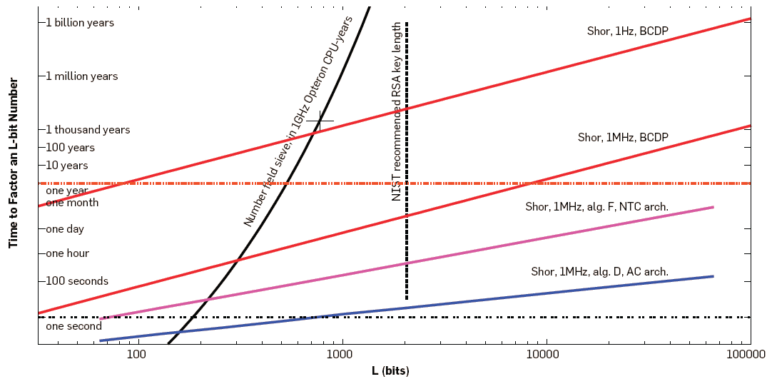
Credit: Figure 1 from A Blueprint For Building a Quantum Computer by Van Meter and Horsman, Communications of the ACM, Oct 2013. Copyright by Van Meter and Horsman and ACM.
Figure 20.1 shows estimated time to factor a L-bit number. The number field sieve on the solid black line is using a classical computer. The cross on that line is for the point of L=768 bits and 3300 CPU years. The NIST recommended key length is L=2048 bits. The lines labelled with Shor are using a quantum computer. The four lines for Shor are different algorithms and architectures, as well as different quantum clock speeds (1Hz vz 1MHz).
One way to read the figure is to look at the number of bits that can be factored in 1 year. A 1GHz classical computer using number field sieve could factor a 500 bit number. A quantum computer using Shor’s algorithm and with a 1 Hz clock could factor a 80 bit number. But with a 1 MHz clock it could factor a 8000 bit number.
Is it likely that quantum computers will break RSA in the near future? Michele Mosca and Marco Piani, from evolutionQ and the Global Risk Institute, interviewed 22 experts in quantum computing, and one question was about the likelihood that quantum computers being a significant threat to public-key cryptosystems in the future.
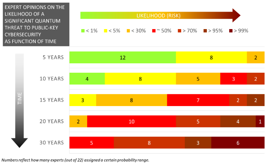
Credit: Quantum Threat Timeline Report, Michele Mosca and Marco Piani, from evolutionQ and the Global Risk Institute, 2019.
Figure 20.2, from the Quantum Threat Timeline Report, shows the opinions of 22 quantum computing experts. Most think quantum computing will not be a threat to public-key cryptosystems in the next 5 years, and more than half, also in the next 10 years. Almost all think there is a 50% or greater chance that quantum computing will threaten RSA in the next 20 years.
20.3 Issues in Quantum Computing
Definition 20.17 (Decoherence in Quantum Computing). In their coherent state, qubits are described as a superposition of states. The loss of coherence (i.e. decoherence) means the qubits revert to their “classical” basis states. They no longer exhibit the unique quantum properties. Decoherence times vary for different system; for example IBM quantum computers about 100 s.
Increasing the time that qubits can hold their coherent state is one practical aim of quantum computing. See the T2 column in the Quantum Computing Report for example values.
Definition 20.18 (Errors in Quantum Computing). Errors frequently occur due to various reasons including: decay of individual qubits; environmental defects that impact multiple qubits; interference between qubits and other systems; accidental measurement of qubits; and even loss of qubits. Significant research effort is on designing error correcting schemes.
Error correcting schemes introduce an overhead, and one concern is that the overhead needed to deal with errors may mean quantum computing does not produce significant advantages over classical computing.
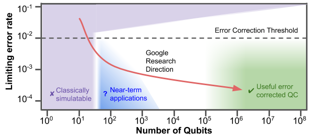
Credit: Google Research, A Preview of Bristlecone, Google’s New Quantum Processor
Figure 20.3, taken from A Preview of Bristlecone, Google’s New Quantum Processor by Google Quantum AI Lab, illustrates the conceptual relationship between error rates and qubits. The error correction threshold indicates error rates below this are needed for error correction to work.
Definition 20.19 (Cooling). For qubits to maintain coherence, quantum circuits need to be very cold, approaching 0 Kelvin or -273 C.
Finally, what are the quantum computers available today?
- For more detailed comparison see the Quantum Computing Report
- Google: Sycamore 53-qubit (2019)
- IBM: 5- and 16-qubit machines available for free; 20-qubit machine available via cloud; 53-qubit machine (2019)
- Rigetti: Aspen-7 28-qubits (2019)
- D-Wave systems: 2000Q has 2048-qubits, however using different technology (quantum annealing) that cannot be used to solve Shor’s algorithm
20.4 Quantum Cryptography
Definition 20.20 (Quantum Cryptography). Quantum cryptography refers to techniques that apply principles of quantum systems to build cryptographic mechanisms. The most widely technique is quantum key distribution. Others approaches often involve agreements between parties that do not trust each other.
Note that while quantum computers can be used to break cryptographic mechanisms (e.g. using Schor’s algorothm), quantum cryptography is separate topic of quantum systems that is about creating cryptographic mechanisms. Quantum cryptographic mechanisms will use quantum computers.
Definition 20.21 (Quantum Key Distribution (informal)). The aim of Quantum Key Distribution (QKD) is for two parties to exchange a secret key (similar to DHKE). A chooses random bits, as well as corresponding random modification of states (called sending basis). Applied together using a fixed scheme, A generates and sends photons in quantum states. B chooses own random measuring basis and measures the photons. A then informs B their sending basis, and allowing B to recognise which of the measured photons to consider (i.e. those where the measuring basis and sending basis match). B uses the resulting bits as a secret key, however only after confirming with A that there are no errors in the key (e.g. sending a challenge encrypted with the key).
For a formal explanation of QKD, with an example see: https://www.cse.wustl.edu/~jain/cse571-07/ftp/quantum/ or the original paper on one scheme BB84 at https://doi.org/10.1016/j.tcs.2014.05.025.
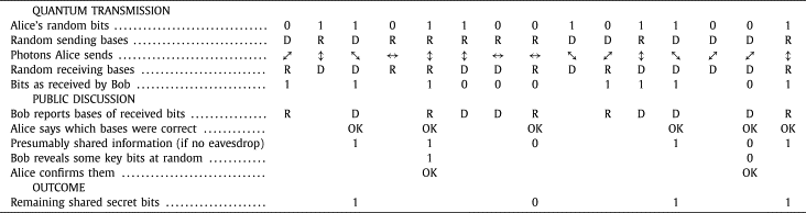
Credit: Bennett and Brassard, Quantum cryptography: Public key distribution and coin tossing, Theoretical Computer Science, Dec 2014, Copyright Elsevier.
Figure 20.4 is taken from the original 1984 article by Bennet and Brassard, which was re-published by Elsevier in the journal Theoretical Computer Science in 2014. BB84 is a scheme still used for quantum key distribution. The paper, in section III, has a nice explanation of the protocol.
Definition 20.22 (QKD security (informal)). An attacker C tries to learn the secret key between A and B, without A or B knowing. Therefore the attacker has to measure the photons sent by A. However, as the photons are a superposition of states, when C measures them, they are changed. As a result, B will receive changed photons, and when they check the secret key with A, the check will fail.
The security of quantum key distribution depends on that measurement problem, i.e. that measuring a quantum superposition state, changes the state. The attacker cannot measure the communications between A and B without changing the communications. It is easy for A and B to recognise if the communications have been changed.
20.5 Cryptography in the Quantum Era
Given that attacks on existing, widely-used ciphers such as RSA may be possible in the (long-term) future using quantum computers, researchers and standardisation organisations are working on ciphers that are resistant to attacks with quantum technologies. This is referred to as post-quantum cryptography.
- NIST Post-Quantum Cryptography project called for proposals on quantum-resistant public key cryptography algorithms
- Digital signatures, public-key encryption, key exchange
- 69 submissions in round 1 (2017)
- 26 algorithms in round 2 (2019)
- 7 finalists in round 3 (2020)
- Plan to standardise in 2022/2023
- Open Quantum Safe has open-source software for prototyping quantum-resistant cryptography, including forks of OpenSSL, OpenSSH and OpenVPN