Converting Coloured Petri Net State Space to Finite State Automata: CPNTools, FSM and Lextools
Formal methods such as Coloured Petri nets can be used to generate the entire set of states of a system being modelled, i.e. an occurrence graph or state space. The state space also shows the entire set of sequences of events that can occur in the system. From this perspective, we can view the state space as a Finite State Machine or Finite State Automata (FSA). Doing so can be benefical as we can then apply well-known algorithms to process the FSA, e.g. to obtain a minimised deterministic FSA and the language accepted by that DFSA. Finally, this process can be used to compare the languages of two different models, e.g. to check if a design model implememts a requirements model or that a protocol offers its desired service.
This is a howto for taking the state space generated from a Coloured Petri net model using the software CPN Tools, converting it into a format such that it is treated as a FSA and can be processed by AT&T's FSM Library, and then generating the language accepted by the FSA. This assumes knowledge of Coloured Petri nets, state spaces, FSA, languages etc, as well as installation and knowledge of CPN Tools (I will show how to install and use parts of FSM Library and Lextools). The steps I show work, but may not be the best. That is, there may be other software available that does the same thing and better suits your needs.
The theory and practice is nothing new, and certainly not developed by me. The steps I show here I used in my PhD thesis 11 years ago. As others have asked how to do it recently, I attempted the steps again (and thankfully, the software and steps still work as they did a decade ago) and outlined them here for future reference. Further description, examples and results of this process are available in my PhD thesis.
Example CPN Model
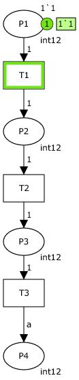
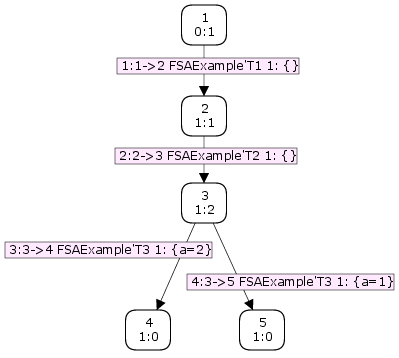
To demonstrate the steps I've created an example, very simple CPN model in CPN Tools version 3.2.2 (running on Windows 7 in a VirtualBox virtual machine with Ubuntu 11.10 host operating system). The example net is below; you can also download the .cpn file to open in CPN Tools. To the right of the model is the state space also generated in CPN Tools:
|
|
The example is just a sequence of three transitions in serial. The declarations in the model are:
colset int12 = int with 1..2;
var a: int12;
Note that the output arc inscription of transition T3 is a, meaning the marking in place P4 may be either 1 or 2.
Saving the State Space as a FSM-Compatible Text File
Writing the State Space to a Text File
Now we need to save the state space in a file that can be processed as a FSA by FSM Library and similar tools. The AT&T FSM Library takes a simple text file as input, where each line contains the source node, destination node and transition (where each are integers). It also has lines with just a single integer, indicating that node is a halt node in the FSA. Therefore in CPN Tools we use the state space exploration Standard ML functions to traverse all the arcs in the state space and printing the source state, destination state and integer representing the arc (more specifically, binding element) to a file. The code I use for this follows. It opens a file, then evaluates function getfsminput (which prints source, destination and arc identifier) on all arcs in the state space, then closes the file.
(* (Arc -> string) -> string -> unit *)
fun og2fsmtrans arc2fsm filename =
let
    val outfile = TextIO.openOut(filename);
    fun getfsminput (a) = TextIO.output(outfile, st_Node(SourceNode(a))^" "^
                                        st_Node(DestNode(a))^" "^
                                        arc2fsm(a)^"\n")
in
    EvalAllArcs(getfsminput);
    TextIO.closeOut(outfile)
end;
The key part of the above function is how to convert arcs in the state space (binding elements) to integers, i.e. the function getfsminput. We'll cover that shortly.
A FSA also needs the set of halt states to be defined. It depends on your model as to what is defined as a halt state. All dead markings in the state space should be halt states, but you may actually have other (live) markings also as halt states. The general function for saving the halt states is:
(* (Node -> bool) -> string -> unit *)
fun og2fsmhalts findhalts filename =
let
    val outfile = TextIO.openOut(filename)
    fun WriteNodes(n) = TextIO.output(outfile, st_Node(n) ^ "\n")
in
    SearchAllNodes(findhalts, fn n => WriteNodes(n),[],op ::);
    TextIO.closeOut(outfile)
end;
You need to supply the function findhalts which must return a list of node numbers that you want to be halt states in the FSA. If you want just dead markings in the state space to be halt states in the FSA then you co do the following:
fun FindHalts n = DeadMarking(n);
If you want something more complex then you must write your own function FindHalts() that takes a state space node as input and returns true if that node is to be a halt state.
Mapping Binding Elements to FSA Transitions
As seen above, the text file representing the FSA will use an integer to represent nodes and transitions. Nodes are easy: CPN Tools also uses integers to identify nodes. Transitions are more complex. The arcs in the state space of a CPN are binding elements. A binding element is the transition that fired and the values of the associated variables. We need to map a binding element (arc in state space) to an integer that represents a transition in the FSA. The exact mapping depends on your model. You could map every different binding element to a distinct integer. In our example state space there are four binding elements. We could map to integers as follows:
- T1 maps to 1
- T2 maps to 2
- T3 with a=1 maps to 3
- T3 with a=2 maps to 4
Of course in non-trivial CPNs there may be a very large number of binding elements. In practice some binding elements may not be of interest. This is especially so when using the output FSA to compare against an existing FSA, for example comparing a protocol specification against its standardised service specification. (Again, my PhD thesis has more detailed explanations and examples of this). Assuming some binding elements are not of interest, then we can map them to an empty transition in the FSA. In the FSA text file an empty transition is represented by the integer 0. For example, lets assume we want to study the ordering of events corresponding with transitions T1 and T3 in our CPN. T2 is of no interest. then we would define the mappings from binding elements to integers as:
- T1 maps to 1
- T2 maps to 0
- T3 with any value of a maps to 2
Now we need to write the arctofsm function used by og2fsmtrans to implement the desired mapping. Lets break it into two functions, the first mapping binding elements to integers (actually strings for output to a file, but the values of the strings are integers):
fun be2str (Bind.FSAExample'T1 (1,_)) = "1"
  | be2str (Bind.FSAExample'T3 (1,_)) = "2"
  | be2str (_) = "0"
The structure Bind returns the binding element on page FSAExample with the first instance of transition T1 with variables bound to any value (represented by _). Any binding element that matches this returns the value "1". Similar for the binding element containing transition T3. For any other binding elements (the last line) the value "0" representing an empty transition is output. I'll refer to the above as mapping 1.
Now since og2fsmtrans operates on all arcs, we use a standard state space ML function to convert arcs to binding elements:
fun ArcToFSM a = be2str(ArcToBE(a));
As a different example, we could have defined the mappings so that the value of a when transition T3 fired was of interest. That is:
fun be2str (Bind.FSAExample'T1 (1,_)) = "1"
  | be2str (Bind.FSAExample'T3 (1,{a=1})) = "2"
  | be2str (Bind.FSAExample'T3 (1,{a=2})) = "3"
  | be2str (_) = "0"
I'll refer to above as mapping 2 and later we will see the difference compared to mapping 1.
Summary
In summary the steps (using mapping 1) are:
- Create CPN model
- Calculate state space
- Define the binding element mappings and halt states
- Execute the following ML code to output the text files
fun be2str (Bind.FSAExample'T1 (1,_)) = "1"
  | be2str (Bind.FSAExample'T3 (1,_)) = "2"
  | be2str (_) = "0"
fun ArcToFSM a = be2str(ArcToBE(a));
fun FindHalts n = DeadMarking(n);
use "og2fsm.sml";
og2fsmtrans ArcToFSM "trans-ex1.txt";
og2fsmhalts FindHalts "halts-ex1.txt";
where I've put the functions og2fsmtrans and og2fsmhalts in the file og2fsm.sml. This should save two text files into your CPN Tools working directory: trans-ex1.txt and halts-ex1.txt.
Installing FSM Library, Lextools and GraphViz
All the above was performing using CPN Tools on Windows (unfortunately the only OS current supported). Now we want to process the FSA (stored in the two text files) using AT&T's FSM Library, Lextools and GraphViz. The latter, GraphViz, is quite a popular graph creation package. FSM Library and Lextools binaries used to be provided freely by AT&T for non-commercial use on their website at http://www.research.att.com/sw/tools/fsm but now it redirects to a page that doesn't include these. It looks like they have a different licensing model for these programs. If you don't have them or have a link to the publicly available packages, let me know.
The binaries for FSM Library and Lextools run in Unix-based operating systems. I'm going to use them on Ubuntu Linux 11.10. Lets first install GraphViz -- its in the repositories (my examples below are copied directly from my terminal so of course you only enter the commands after the $):
sgordon@lime:~/cpn$ sudo apt-get install graphviz
Now lets extract the archives for FSM Library and Lextools:
sgordon@lime:~/cpn$ ls
fsm-4_0.linux.i386.tar.gz  lextools.linux.i386.tar.gz
sgordon@lime:~/cpn$ tar xzf fsm-4_0.linux.i386.tar.gz
sgordon@lime:~/cpn$ tar xzf lextools.linux.i386.tar.gz
sgordon@lime:~/cpn$ ls
bin-i686  fsm-4.0  fsm-4_0.linux.i386.tar.gz  lextools-3  lextools.linux.i386.tar.gz  man  README
Binaries and man pages for FSM Library are in the fsm-4.0 directory. You can manually copy them to a directory in your path. For Lextools they are in bin-i686 and man directories, and some additional files are in lextools-3. Again you need to manually copy them, as explained in the README. In my case I'm going to put all binaries in /usr/local/bin/, the man pages in the appropriate sub-directories of /usr/local/man/ and the Lextools library files in /usr/local/lib/lextools-3/:
sgordon@lime:~/cpn$ echo $PATH
/usr/lib/lightdm/lightdm:/usr/local/sbin:/usr/local/bin:/usr/sbin:/usr/bin:/sbin:/bin:/usr/games
sgordon@lime:~/cpn$ sudo cp fsm-4.0/bin/* /usr/local/bin/
sgordon@lime:~/cpn$ sudo mkdir -p /usr/local/man/man1
sgordon@lime:~/cpn$ sudo mkdir -p /usr/local/man/man3
sgordon@lime:~/cpn$ sudo mkdir -p /usr/local/man/man5
sgordon@lime:~/cpn$ sudo cp fsm-4.0/doc/f*.1 /usr/local/man/man1/
sgordon@lime:~/cpn$ sudo cp fsm-4.0/doc/f*.3 /usr/local/man/man3/
sgordon@lime:~/cpn$ sudo cp fsm-4.0/doc/f*.5 /usr/local/man/man5/
sgordon@lime:~/cpn$ sudo cp bin-i686/* /usr/local/bin/
sgordon@lime:~/cpn$ sudo cp man/lextools.1 /usr/local/man/man1/
sgordon@lime:~/cpn$ sudo cp man/lextools.5 /usr/local/man/man5/
sgordon@lime:~/cpn$ sudo mkdir /usr/local/lib/lextools-3/Fragments
sgordon@lime:~/cpn$ sudo mkdir /usr/local/lib/lextools-3/grammars
sgordon@lime:~/cpn$ sudo cp lextools-3/lib/Fragments/* /usr/local/lib/lextools-3/Fragments/
sgordon@lime:~/cpn$ sudo cp lextools-3/grammars/* /usr/local/lib/lextools-3/grammars/
Now lets test by viewing the man page of several commands (the -S5 option should should the man page aboit file formats for Lextools) and trying fsmcompile:
sgordon@lime:~/cpn$ man fsm
sgordon@lime:~/cpn$ man lextools
sgordon@lime:~/cpn$ man -S5 lextools
sgordon@lime:~/cpn$ fsmcompile
^C
sgordon@lime:~/cpn$
If fsmcompile does NOT return a command not found error then it should be ok.
Minimising the NDFSA and Language Generation
There are many commands available in the FSM Library and Lextools packages. Here I am going to demonstrate taking our non-deterministic FSA created from the state space and reduce it to a minimised deterministic FSA and the language it accepts. Then use GraphViz (specifically, dot) to produce a image showing the FSA. I will not explain the steps for FSA minimization (read a textbook such as ) nor the exact commands (read the man pages). The assumptions is that the trans-ex1.txt and halts-ex1.txt files existing in your working directory (in example below) AND you have an additional file that maps the integer transitions to meaningful names. In this case called labels-ex1.txt.
sgordon@lime:~/example$ ls
halts-ex1.txt  halts-ex2.txt  labels-ex1.txt  labels-ex2.txt  trans-ex1.txt  trans-ex2.txt
sgordon@lime:~/example$ cat trans-ex1.txt halts-ex1.txt > ex1-ss.txt
sgordon@lime:~/example$ fsmcompile ex1-ss.txt > ex1-ss.fsm
sgordon@lime:~/example$ fsmrmepsilon ex1-ss.fsm > ex1-ssnoeps.fsm
sgordon@lime:~/example$ fsmdeterminize ex1-ssnoeps.fsm > ex1-ssdeterm.fsm
sgordon@lime:~/example$ fsmminimize ex1-ssdeterm.fsm > ex1-ssmin.fsm
sgordon@lime:~/example$ fsminfo -n ex1-ssmin.fsm
class                   	basic
semiring                	tropical
transducer              	n
# of states             	3
# of arcs               	2
initial state           	0
# of final states       	1
# of eps                	0
# of accessible states  	3
# of coaccessible states	3
# of connected states   	3
# strongly conn components	3

sgordon@lime:~/example$ lexfsmstrings -l labels-ex1.txt ex1-ssmin.fsm > ex1-lang.txt
sgordon@lime:~/example$ cat ex1-lang.txt
[Transition1][Transition3]
sgordon@lime:~/example$ fsmdraw -f 32 -t '' -i labels-ex1.txt ex1-ssmin.fsm > ex1-ssdraw.txt
sgordon@lime:~/example$ dot -Tps -o ex1-ssdraw.ps ex1-ssdraw.txt
sgordon@lime:~/example$ ps2pdf ex1-ssdraw.ps
Two things outputs worth mentioning. The language accepted by the FSA is stored in the ex1-lang.txt file. Each line shows a sequence of transitions that are possible. In our example, only one such sequence exists. The other file is the PDF that shows the FSA.
The above example was using mapping 1. I've repeated the steps using mapping 2 (files named ex2 instead of ex1) and the converted the output PDFs to PNGs as below:
 |
 |
| FSA using Mapping 1 | FSA using Mapping 2 |
We see now the impact of the different binding element mappings.
All the files (for both mappings) including the CPN model and intermediate FSM files are available for download as an TGZ archive: fsa-example.tgz.
Created on Mon, 20 Feb 2012, 5:37pm
Last changed on Fri, 16 Aug 2013, 11:50am